DAV Question Paper solution Dec 2023

DAV Question Paper solution Dec 2023

download as an pdf :

https://drive.google.com/file/d/1ii57ewWx1IrbSarEgfZ9M6cWz7-md59p/view?usp=sharing

Q1. Attempt the following (any 4): (20) DAV Question Paper solution Dec 2023

a. Why is data analytics lifecycle essential?

https://www.rudderstack.com/learn/data-analytics/data-analytics-lifecycle

b. The regression lines of a sample are x +6y=6 and 3x+2y=10
Find (i) sample means x and y
(ii) coefficient of correlation between x and y

Please add an Answer or view existing answer for this question : https://www.doubtly.in/q/regression-lines-sample-6y6-3x2y10/

c. Differentiate between linear regression and logistic regression.

Feature	Linear Regression	Logistic Regression
Type of Prediction	Predicts continuous numerical outcomes.	Predicts categorical outcomes (binary or multi-class)
Output Range	Unbounded (can be any real number).	Bounded between 0 and 1 (probability).
Nature of Output	Dependent variable is continuous.	Dependent variable is categorical.
Equation Type	Linear equation.	Logistic (Sigmoid) function.
Example Usage	Predicting house prices, stock prices.	Predicting whether an email is spam or not.
Error Measurement	Typically uses Mean Squared Error (MSE) or similar.	Typically uses Log Loss or Cross-Entropy Loss.
Assumption about Errors	Assumes errors are normally distributed.	Assumes errors follow a Bernoulli distribution.
Model Interpretability	Easily interpretable, coefficients indicate impact.	Less interpretable, coefficients represent log odds.
Complexity	Less complex.	More complex due to non-linear transformation.
Overfitting Concerns	More prone to overfitting.	Less prone to overfitting due to regularization.
Handling Outliers	Sensitive to outliers, can significantly affect model.	Less sensitive to outliers due to logistic function.
Applications	Prediction of quantities (sales, temperature).	Classification tasks (spam detection, churn prediction).

d. What is Pandas? State and explain key features of Pandas.

Pandas is a powerful open-source data manipulation and analysis library for Python. It provides easy-to-use data structures and data analysis tools, making it a fundamental tool for data analytics and manipulation in Python. Here are some key features of Pandas:

1. DataFrame: Pandas introduces the DataFrame, a two-dimensional labeled data structure with columns of potentially different types. It is similar to a spreadsheet or SQL table, where data can be easily manipulated and analyzed. DataFrames allow for easy indexing, slicing, and reshaping of data.
2. Series: Pandas also offers a Series data structure, which is a one-dimensional labeled array capable of holding any data type. Series are the building blocks of DataFrames, representing columns or rows of data.
3. Data Manipulation: Pandas provides a wide range of functions and methods for data manipulation, including merging, joining, grouping, sorting, filtering, and aggregating data. These operations enable users to clean, transform, and preprocess data efficiently.
4. Missing Data Handling: Pandas offers robust support for handling missing or null values in datasets. It provides methods for detecting, removing, and filling missing data, allowing for cleaner and more accurate analysis.
5. IO Tools: Pandas supports reading and writing data from various file formats, including CSV, Excel, SQL databases, JSON, HTML, and more. This makes it easy to import data from external sources and export results to different formats.
6. Data Alignment and Arithmetic Operations: Pandas aligns data based on index labels, enabling easy arithmetic operations between DataFrames and Series. This feature simplifies calculations and data manipulation, especially when working with datasets of different shapes.
7. Time Series Analysis: Pandas includes powerful tools for working with time series data. It provides date/time indexing, resampling, shifting, rolling window operations, and other functionalities essential for time-based analysis and visualization.
8. Visualization: Pandas integrates with other Python libraries like Matplotlib and Seaborn to facilitate data visualization. It offers convenient plotting functions for generating various types of charts and graphs directly from DataFrame and Series objects.
9. Efficiency and Performance: Pandas is optimized for speed and efficiency, with many operations implemented in highly optimized C or Cython code. It can handle large datasets efficiently, making it suitable for both exploratory analysis and production-level applications.
10. Integration with NumPy and SciPy: Pandas seamlessly integrates with other essential data science libraries like NumPy and SciPy. This interoperability allows users to leverage the capabilities of these libraries for advanced numerical computation, statistical analysis, and scientific computing.

e. Explain term frequency (TF), document frequency (DF), and inverse document frequency (IDF)

Term Frequency (TF), Document Frequency (DF), and Inverse Document Frequency (IDF) are concepts commonly used in natural language processing and information retrieval for text analysis.

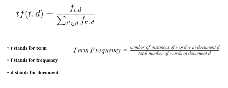
Term Frequency (TF):

• Term Frequency refers to the frequency of occurrence of a term (word) within a document.
• It measures how often a term appears in a document relative to the total number of terms in that document.
• TF is calculated using the following formula:

Document Frequency (DF):

• Document Frequency indicates how many documents contain a particular term.
• It measures the frequency of occurrence of a term across the entire corpus (collection of documents).
• DF is calculated by counting the number of documents in which a term occurs at least once.
• It is useful for determining the importance of a term in the context of the entire corpus.

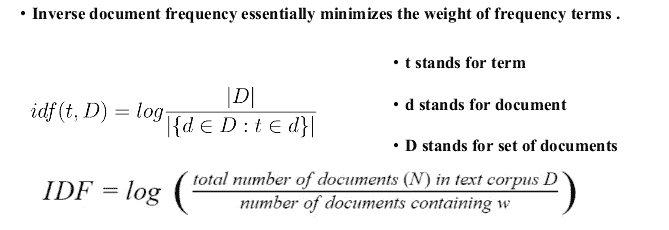
Inverse Document Frequency (IDF):

• Inverse Document Frequency is a measure of how unique or rare a term is across all documents in the corpus.
• It is calculated by taking the logarithm of the ratio of the total number of documents to the document frequency of the term.
• IDF assigns higher weights to terms that are rare across the corpus and lower weights to terms that are common.
• It is particularly useful for highlighting the significance of terms that occur infrequently but are highly informative.
• IDF is calculated using the following formula:

The combination of TF and IDF is often used to compute a weight for each term in a document, known as TF-IDF (Term Frequency-Inverse Document Frequency). TF-IDF assigns a higher weight to terms that are frequent within a document (high TF) but rare across the corpus (high IDF), making it a useful metric for text mining tasks such as document classification, information retrieval, and keyword extraction.

Q2. Attempt the following:

a. Explain the data analytics lifecycle. (10) (repeated question)

Data Analytics Lifecycle :
The Data analytic lifecycle is designed for Big Data problems and data science projects. The cycle is iterative to represent real project. To address the distinct requirements for performing analysis on Big Data, step – by – step methodology is needed to organize the activities and tasks involved with acquiring, processing, analyzing, and repurposing data.

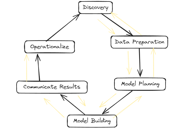
Phase 1: Discovery –

• The data science team learn and investigate the problem.
• Develop context and understanding.
• Come to know about data sources needed and available for the project.
• The team formulates initial hypothesis that can be later tested with data.

Phase 2: Data Preparation –

• Steps to explore, preprocess, and condition data prior to modeling and analysis.
• It requires the presence of an analytic sandbox, the team execute, load, and transform, to get data into the sandbox.
• Data preparation tasks are likely to be performed multiple times and not in predefined order.
• Several tools commonly used for this phase are – Hadoop, Alpine Miner, Open Refine, etc.

Phase 3: Model Planning –

• Team explores data to learn about relationships between variables and subsequently, selects key variables and the most suitable models.
• In this phase, data science team develop data sets for training, testing, and production purposes.
• Team builds and executes models based on the work done in the model planning phase.
• Several tools commonly used for this phase are – Matlab, STASTICA.

Phase 4: Model Building –

• Team develops datasets for testing, training, and production purposes.
• Team also considers whether its existing tools will suffice for running the models or if they need more robust environment for executing models.
• Free or open-source tools – Rand PL/R, Octave, WEKA.
• Commercial tools – Matlab , STASTICA.

Phase 5: Communication Results –

• After executing model team need to compare outcomes of modeling to criteria established for success and failure.
• Team considers how best to articulate findings and outcomes to various team members and stakeholders, taking into account warning, assumptions.
• Team should identify key findings, quantify business value, and develop narrative to summarize and convey findings to stakeholders.

Phase 6: Operationalize –

• The team communicates benefits of project more broadly and sets up pilot project to deploy work in controlled way before broadening the work to full enterprise of users.
• This approach enables team to learn about performance and related constraints of the model in production environment on small scale , and make adjustments before full deployment.
• The team delivers final reports, briefings, codes.
• Free or open source tools – Octave, WEKA, SQL, MADlib.

b. Find two lines of regression from the following data: (10)

Age of Husband (x)	25	22	28	26	35	20	22	40	20	18
Age of wife (y)	18	15	20	17	22	14	16	21	15	14

Estimate (i) the age of husband when the age of wife is 19 and (ii) the age of wife when
the age of the husband is 30

Answer : https://www.doubtly.in/q/find-lines-regression-data/

Q3 Attempt the following:

a. Explain Box-Jenkins intervention analysis.

Answer : https://www.doubtly.in/q/explain-box-jenkins-intervention-analysis/

b. What is text mining? Enlist and explain the seven practice areas of text analytics

Text mining, also known as text analytics, is the process of deriving meaningful information from natural language text. It involves various techniques from linguistics, computer science, and statistics to extract patterns, trends, and insights from unstructured text data.

The seven practice areas of text analytics are:

1. Text Classification:
   • Text classification involves categorizing documents into predefined categories or classes based on their content. It is commonly used for sentiment analysis, spam detection, topic categorization, and more.
   • Techniques used in text classification include machine learning algorithms such as Naive Bayes, Support Vector Machines (SVM), and deep learning models like Convolutional Neural Networks (CNN) and Recurrent Neural Networks (RNN).
2. Text Clustering:
   • Text clustering involves grouping similar documents together based on their content without predefined categories. It helps in exploring the underlying structure of large text collections and identifying themes or topics.
   • Clustering algorithms like K-means, hierarchical clustering, and DBSCAN are commonly used in text clustering.
3. Information Extraction:
   • Information extraction focuses on identifying and extracting structured information from unstructured text, such as named entities, relationships, and events. This information is then organized into a structured format for further analysis.
   • Techniques include Named Entity Recognition (NER), relation extraction, and event extraction, often combined with machine learning algorithms.
4. Sentiment Analysis:
   • Sentiment analysis aims to determine the sentiment or opinion expressed in a piece of text, whether it’s positive, negative, or neutral. It is widely used in social media monitoring, customer feedback analysis, and brand reputation management.
   • Approaches to sentiment analysis include lexicon-based methods, machine learning models (e.g., Support Vector Machines, Recurrent Neural Networks), and hybrid approaches.
5. Topic Modeling:
   • Topic modeling is a statistical technique for discovering abstract topics or themes present in a collection of documents. It helps in uncovering the underlying structure of large text corpora and understanding the main themes discussed.
   • Popular topic modeling algorithms include Latent Dirichlet Allocation (LDA) and Non-negative Matrix Factorization (NMF).
6. Text Summarization:
   • Text summarization involves automatically generating concise and coherent summaries of longer texts while preserving the most important information. It is useful for condensing large documents, news articles, or research papers.
   • Techniques for text summarization include extractive methods (e.g., selecting and combining important sentences) and abstractive methods (e.g., generating new sentences to convey the main ideas).
7. Text Generation:
   • Text generation focuses on automatically producing human-like text based on a given input or context. It includes tasks like machine translation, dialogue generation, and story generation.
   • Techniques range from rule-based systems to advanced deep learning models such as Generative Adversarial Networks (GANs) and Transformers.

Q4. Attempt the following:

a. Explain different types of data visualizations in R programming language.

In R programming language, there are various types of data visualizations that can be created using different packages such as ggplot2, plotly, ggvis, lattice, and base R graphics. Here are some common types of data visualizations in R:

1. Scatter Plots:

• Scatter plots are used to visualize the relationship between two continuous variables. Each data point is represented as a dot, and the position of the dot on the plot indicates the values of the two variables.
• Example code using ggplot2:
  R library(ggplot2) ggplot(data = iris, aes(x = Sepal.Length, y = Sepal.Width)) + geom_point()

1. Bar Plots:

• Bar plots are used to visualize the distribution or comparison of categorical variables. They represent the frequency or proportion of each category with rectangular bars.
• Example code using ggplot2:
  R ggplot(data = iris, aes(x = Species)) + geom_bar()

1. Histograms:

• Histograms are used to visualize the distribution of a single continuous variable. They divide the range of values into bins and display the frequency or density of observations within each bin.
• Example code using ggplot2:
  R ggplot(data = iris, aes(x = Sepal.Length)) + geom_histogram(binwidth = 0.5)

1. Line Plots:

• Line plots are used to visualize trends or patterns in data over time or any other ordered variable. They connect data points with straight lines.
• Example code using ggplot2:
  R ggplot(data = economics, aes(x = date, y = unemploy)) + geom_line()

1. Box Plots:

• Box plots (also known as box-and-whisker plots) are used to visualize the distribution of a continuous variable across different categories. They display the median, quartiles, and outliers of the data.
• Example code using ggplot2:
  R ggplot(data = iris, aes(x = Species, y = Sepal.Length)) + geom_boxplot()

1. Heatmaps:

• Heatmaps are used to visualize the magnitude of a variable across two dimensions (e.g., time and categories) using colors. They are often used to represent correlation matrices or density plots.
• Example code using ggplot2:
  R ggplot(data = mtcars, aes(x = factor(cyl), y = factor(vs))) + geom_tile(aes(fill = mpg))

1. Scatterplot Matrices:

• Scatterplot matrices are used to visualize pairwise relationships between multiple variables in a dataset. They consist of grids of scatter plots, with each plot showing the relationship between two variables.
• Example code using ggplot2:
  R library(GGally) ggpairs(data = iris[, 1:4])

These are just a few examples of the types of visualizations you can create in R. Depending on your data and the insights you want to extract, you can choose the most appropriate type of visualization to effectively communicate your findings.

b. Fit a regression equation to estimate β0 ,β1 and β2 to the following data of a transport
company on the weights of 6 shipments, the distances they were moved and the damage
of the goods that was incurred. (10)

Weight X1 (1000)	4.0	3.0	1.6	1.2	3.4	4.8
Distance X2 (100KM)	1.5	2.2	1.0	2.0	0.8	1.6
Damage Y (Rs)	160	112	69	90	123	186

Estimate the damage when a shipment of 3700 kg is moved to a distance of 260 km

Answer : https://www.doubtly.in/q/fit-regression-equation-estimate-%ce%b20-%ce%b21-%ce%b22/

Q5. Attempt the following:

a. From the following results, obtain two regression equations and estimate the yield
when the rainfall is 29 cm and the rainfall when the yield is 600 kg. (10)

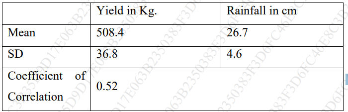
Answer : https://www.doubtly.in/q/estimate-yield-rainfall-29-cm-rainfall-yield-600-kg/

b. What is stepwise regression? State and explain different types of stepwise regression

Stepwise regression is a method used in statistical modeling to select a subset of predictor variables (independent variables) for a regression model. The main idea behind stepwise regression is to iteratively add or remove predictor variables from the model based on their statistical significance or contribution to the model’s predictive power. This process continues until a stopping criterion is met, such as reaching a predefined significance level or finding the best-performing model according to a chosen criterion (e.g., AIC, BIC).

There are typically two main types of stepwise regression:

1. Forward Selection:

• In forward selection, the algorithm starts with an empty model (no predictor variables) and iteratively adds one predictor variable at a time.
• At each step, the algorithm evaluates the contribution of each remaining predictor variable to the model using a predefined criterion (e.g., p-value, information criterion).
• The variable with the most significant contribution (e.g., lowest p-value) is added to the model, and the process continues until no remaining variables meet the inclusion criterion.

1. Backward Elimination:

• In backward elimination, the algorithm starts with a model containing all predictor variables.
• At each step, the algorithm evaluates the contribution of each predictor variable to the model using a predefined criterion.
• The variable with the least significant contribution (e.g., highest p-value) is removed from the model, and the process continues until no variable meets the elimination criterion.

Additionally, there is a variant known as Bidirectional Elimination or Stepwise Regression with Both Directions:

• Bidirectional elimination combines elements of both forward selection and backward elimination.
• It starts with an empty model and alternates between forward selection (adding variables) and backward elimination (removing variables) until no further improvements are possible or until a stopping criterion is met.

Stepwise regression methods are commonly used for variable selection in situations where there are many potential predictor variables, and the goal is to identify the most relevant subset of variables for building a parsimonious and interpretable regression model. However, caution should be exercised when using stepwise regression, as it can lead to overfitting or selecting spurious variables if not performed carefully.

Q6. Write short notes on (any 2):

a. Time Series Analysis:

• Time series analysis deals with analyzing data points collected, recorded, or observed at consecutive time intervals.
• It focuses on understanding the underlying patterns, trends, and behaviors exhibited by the data over time.
• Techniques like smoothing, decomposition, autocorrelation analysis, and forecasting are commonly employed in time series analysis.
• Applications include economic forecasting, stock market analysis, weather prediction, and signal processing.

b. Exploratory Data Analysis (EDA):

• Exploratory Data Analysis is a crucial step in the data analysis process that involves summarizing the main characteristics of a dataset.
• It aims to gain insights into the data, identify patterns, spot anomalies, and formulate hypotheses for further investigation.
• Techniques used in EDA include summary statistics, data visualization (e.g., histograms, scatter plots), and correlation analysis.
• EDA helps in understanding the structure of the data and guiding subsequent analysis or modeling efforts.

c. Regression Plot:

• A regression plot is a graphical representation of the relationship between two variables in a regression analysis.
• It typically involves plotting the observed data points along with the fitted regression line.
• Regression plots are useful for visually assessing the strength and direction of the relationship between the variables.
• They can also help in identifying outliers or influential data points that might affect the regression model’s performance.

d. Generalized Linear Model (GLM):

• The Generalized Linear Model is a flexible framework for modeling the relationship between a response variable and one or more predictor variables.
• It extends the linear regression model by allowing the response variable to have a distribution other than the normal distribution and by using a link function to relate the mean of the response variable to the predictors.
• GLM accommodates various types of response variables, including binary (logistic regression), count (Poisson regression), and categorical (multinomial regression).
• GLM is widely used in fields such as biostatistics, econometrics, and social sciences for modeling non-normal data distributions and handling diverse types of response variables.