DAV Question Paper solution May 2023

download as an pdf :

https://drive.google.com/file/d/1ii57ewWx1IrbSarEgfZ9M6cWz7-md59p/view?usp=sharing

DAV Question Paper solution May 2023 , some of the answers have an link , if you know the answer please add an solution to it

Q1

a) What is an analytic sandbox, and why is it important ?

An analytical sandbox is a testing environment that is used by data analysts and data scientists to experiment with data and explore various analytical approaches without affecting the production environment. It is a separate, isolated environment that contains a copy of the production data, as well as the necessary tools and resources for data analysis and visualization.

Analytical sandboxes are typically used for a variety of purposes, including testing and validating new analytical approaches and algorithms, trying out different data sets, collaborating and sharing work with colleagues, and testing new data visualization techniques and dashboards.

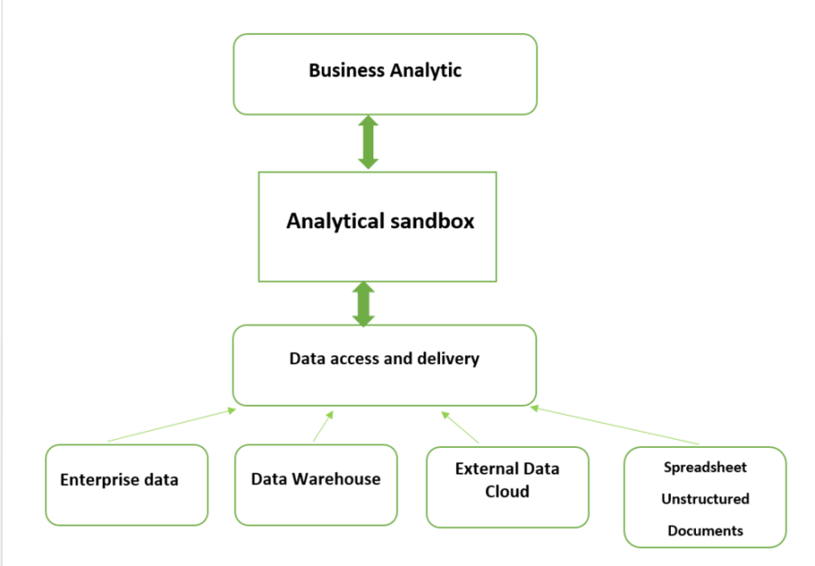
Analytical Sandbox’s Essential Components Include:

1. Business Analytics (Enterprise Analytics) – The self-service BI tools for situational analysis and discovery are part of business analytics.
2. Analytical Sandbox Platform – The capabilities for processing, storing, and networking are provided by the analytical sandbox platform.
3. Data Access and Delivery – Data collection and integration are made possible by data access and delivery from a number of data sources and data kinds.
4. Data Sources – Big data (unstructured) and transactional data (structured) are two types of data sources that can come from both inside and outside of the company. Examples of these sources include extracts, feeds, messages, spreadsheets, and documents.

Graphical view of Analytical Sandbox Components

Importance of an Analytical Sandbox

1. Data from various sources, both internal and external, both unstructured and structured, can be combined and filtered using analytical sandboxes.
2. Data scientists can carry out complex analytics with the help of analytical sandboxes.
3. Analytical sandboxes enable working with data initially.
4. Analytical sandboxes make it possible to use high-performance computing while processing databases because the analytics takes place inside the database itself.

b) Why use autocorrelation instead of autocovariance when examining stationary  time series?

Autocorrelation and autocovariance are one of the most critical metrics in financial time series econometrics. Both functions are based on covariance and correlation metrics.

What is Autocorrelation? Autocorrelation measures the degree of similarity between a given time series and the lagged version of that time series over successive time periods. It is similar to calculating the correlation between two different variables except in Autocorrelation we calculate the correlation between two different versions Xt and Xt-k of the same time series.

What is Autocovariance? Autocovariance is defined as the covariance between the present value (xt) with the previous value (xt-1) and the present value (xt) with (xt-2). And it is denoted as γ. In a stationary time series, data are challenging and are likely to change considering the assumptions of linear programming. In such a situation, the residual errors can be correlated in order to eliminate inconsistency. When the autocovariance is utilized, its variables can change over time which can lead to invalid results.

In stationary time series, the statistical properties of the data do not change considerably over time. Hence autocorrelation will be much applicable when compared to autocovariance.

c) Difference between Pandas and NumPy.

Answer : https://www.doubtly.in/q/difference-pandas-numpy/

d) What is regression? What is simple linear regression?

Answer : https://www.doubtly.in/q/regression-simple-linear-regression/

Q2 a) Explain in detail how dirty data can be detected in the data exploration phase  with visualizations. 

Answer will be added here : https://www.doubtly.in/q/explain-detail-dirty-data-detected/

Q2 b) List and explain methods that can be used for sentiment analysis.

Sentiment analysis is the process of identifying and extracting subjective information from text, such as opinions and emotions. 

There are several methods that can be used for sentiment analysis, including: 

1. Lexicon-based methods: In this method, sentiment scores are assigned to words based on their dictionary meanings. The sentiment scores are then aggregated to produce an overall sentiment score for a piece of text. 

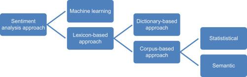
The different approaches to lexicon-based approach are:

Dictionary-based approach

In this approach, a dictionary is created by taking a few words initially. Then an online dictionary, thesaurus or WordNet can be used to expand that dictionary by incorporating synonyms and antonyms of those words. The dictionary is expanded till no new words can be added to that dictionary. The dictionary can be refined by manual inspection.

 Corpus-based approach

This finds sentiment orientation of context-specific words. The two methods of this approach are:

• Statistical approach: The words which show erratic behavior in positive behavior are considered to have positive polarity. If they show negative recurrence in negative text they have negative polarity. If the frequency is equal in both positive and negative text then the word has neutral polarity.
• Semantic approach: This approach assigns sentiment values to words and the words which are semantically closer to those words; this can be done by finding synonyms and antonyms with respect to that word.

2. Machine learning-based methods: In this method, a machine learning algorithm is trained on a labeled dataset to predict the sentiment of a given piece of text. The algorithm can then be used to classify new text as positive, negative, or neutral. 
3. Hybrid methods: These methods combine lexicon-based and machine learning-based methods to improve the accuracy of sentiment analysis. 
4. Rule-based methods: In this method, a set of rules are defined to identify sentiment in a piece of text. The rules may be based on linguistic rules or domain-specific rules. The choice of method depends on the specific requirements of the analysis, the quality and quantity of data, and the available resources.

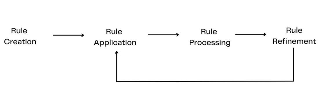
Steps in Rule-based approach:

1. Rule Creation: Based on the desired tasks, domain-specific linguistic rules are created such as grammar rules, syntax patterns, semantic rules or regular expressions.
2. Rule Application: The predefined rules are applied to the inputted data to capture matched patterns.
3. Rule Processing: The text data is processed in accordance with the results of the matched rules to extract information, make decisions or other tasks.
4. Rule refinement: The created rules are iteratively refined by repetitive processing to improve accuracy and performance. Based on previous feedback, the rules are modified and updated when needed.

Q3 a) List and explain the main phases of the Data Analytics Lifecycle.

Data Analytics Lifecycle :
The Data analytic lifecycle is designed for Big Data problems and data science projects. The cycle is iterative to represent real project. To address the distinct requirements for performing analysis on Big Data, step – by – step methodology is needed to organize the activities and tasks involved with acquiring, processing, analyzing, and repurposing data.

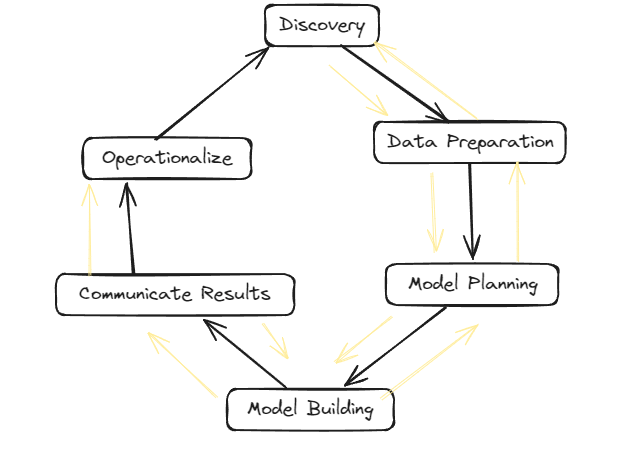
Phase 1: Discovery –

• The data science team learn and investigate the problem.
• Develop context and understanding.
• Come to know about data sources needed and available for the project.
• The team formulates initial hypothesis that can be later tested with data.

Phase 2: Data Preparation –

• Steps to explore, preprocess, and condition data prior to modeling and analysis.
• It requires the presence of an analytic sandbox, the team execute, load, and transform, to get data into the sandbox.
• Data preparation tasks are likely to be performed multiple times and not in predefined order.
• Several tools commonly used for this phase are – Hadoop, Alpine Miner, Open Refine, etc.

Phase 3: Model Planning –

• Team explores data to learn about relationships between variables and subsequently, selects key variables and the most suitable models.
• In this phase, data science team develop data sets for training, testing, and production purposes.
• Team builds and executes models based on the work done in the model planning phase.
• Several tools commonly used for this phase are – Matlab, STASTICA.

Phase 4: Model Building –

• Team develops datasets for testing, training, and production purposes.
• Team also considers whether its existing tools will suffice for running the models or if they need more robust environment for executing models.
• Free or open-source tools – Rand PL/R, Octave, WEKA.
• Commercial tools – Matlab , STASTICA.

Phase 5: Communication Results –

• After executing model team need to compare outcomes of modeling to criteria established for success and failure.
• Team considers how best to articulate findings and outcomes to various team members and stakeholders, taking into account warning, assumptions.
• Team should identify key findings, quantify business value, and develop narrative to summarize and convey findings to stakeholders.

Phase 6: Operationalize –

• The team communicates benefits of project more broadly and sets up pilot project to deploy work in controlled way before broadening the work to full enterprise of users.
• This approach enables team to learn about performance and related constraints of the model in production environment on small scale , and make adjustments before full deployment.
• The team delivers final reports, briefings, codes.
• Free or open source tools – Octave, WEKA, SQL, MADlib.

Q3 b) Describe how logistic regression can be used as a classifier.

• Logistic regression is one of the most popular Machine Learning algorithms, which comes under the Supervised Learning technique. It is used for predicting the categorical dependent variable using a given set of independent variables.
• Logistic regression predicts the output of a categorical dependent variable. Therefore the outcome must be a categorical or discrete value. It can be either Yes or No, 0 or 1, true or False, etc. but instead of giving the exact value as 0 and 1, it gives the probabilistic values which lie between 0 and 1.
• Logistic Regression is much similar to the Linear Regression except that how they are used. Linear Regression is used for solving Regression problems, whereas Logistic regression is used for solving the classification problems.
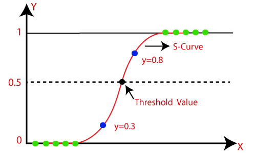
• In Logistic regression, instead of fitting a regression line, we fit an “S” shaped logistic function, which predicts two maximum values (0 or 1).
• The curve from the logistic function indicates the likelihood of something such as whether the cells are cancerous or not, a mouse is obese or not based on its weight, etc.
• Logistic Regression is a significant machine learning algorithm because it has the ability to provide probabilities and classify new data using continuous and discrete datasets.
• Logistic Regression can be used to classify the observations using different types of data and can easily determine the most effective variables used for the classification. The below image is showing the logistic function:

Why do we use Logistic Regression rather than Linear Regression?

• Logistic regression is only used when our dependent variable is binary and in linear regression this dependent variable is continuous.
• The second problem is that if we add an outlier in our dataset, the best fit line in linear regression shifts to fit that point.
• Now, if we use linear regression to find the best fit line which aims at minimizing the distance between the predicted value and actual value, the line will be like this:
• Here the threshold value is 0.5, which means if the value of h(x) is greater than 0.5 then we predict malignant tumor (1) and if it is less than 0.5 then we predict benign tumor (0). 
• Everything seems okay here but now let’s change it a bit, we add some outliers in our dataset, now this best fit line will shift to that point. Hence the line will be somewhat like this:

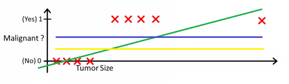
• The blue line represents the old threshold and the yellow line represents the new threshold which is maybe 0.2 here. 
• To keep our predictions right we had to lower our threshold value. Hence we can say that linear regression is prone to outliers. 
• Now here if h(x) is greater than 0.2 then only this regression will give correct outputs.
• Another problem with linear regression is that the predicted values may be out of range. 
• We know that probability can be between 0 and 1, but if we use linear regression this probability may exceed 1 or go below 0.
• To overcome these problems we use Logistic Regression, which converts this straight best fit line in linear regression to an S-curve using the sigmoid function, which will always give values between 0 and 1. 

Q4 a) Suppose everyone who visits a retail website gets one promotional offer or no promotion at all. We want to see if making a promotional offer makes a  difference. What statistical method would you recommend for this analysis? 

Q4 b) List and explain the steps in the Text Analysis.

Language Identification

• Objective: Determine the language in which the text is written.
• How it works: Algorithms analyze patterns within the text to identify the language. This is essential for subsequent processing steps, as different languages may have different rules and structures.

Tokenization

• Objective: Divide the text into individual units, often words or sub-word units (tokens).
• How it works: Tokenization breaks down the text into meaningful units, making it easier to analyze and process. It involves identifying word boundaries and handling punctuation.

Sentence Breaking

• Objective: Identify and separate individual sentences in the text.
• How it works: Algorithms analyze the text to determine where one sentence ends and another begins. This is crucial for tasks that require understanding the context of sentences.

Part of Speech Tagging

• Objective: Assign a grammatical category (part of speech) to each token in a sentence.
• How it works: Machine learning models or rule-based systems analyze the context and relationships between words to assign appropriate part-of-speech tags (e.g., noun, verb, adjective) to each token.

Chunking

• Objective: Identify and group related words (tokens) together, often based on the part-of-speech tags.
• How it works: Chunking helps in identifying phrases or meaningful chunks within a sentence. This step is useful for extracting information about specific entities or relationships between words.

Syntax Parsing

• Objective: Analyze the grammatical structure of sentences to understand relationships between words.
• How it works: Syntax parsing involves creating a syntactic tree that represents the grammatical structure of a sentence. This tree helps in understanding the syntactic relationships and dependencies between words.

Sentence Chaining

• Objective: Connect and understand the relationships between multiple sentences.
• How it works: Algorithms analyze the content and context of different sentences to establish connections or dependencies between them. This step is crucial for tasks that require a broader understanding of the text, such as summarization or document-level sentiment analysis.

Q5 a) How does the ARMA model differ from the ARIMA model? In what situation is  the ARMA model appropriate? 

The ARMA (AutoRegressive Moving Average) model and the ARIMA (AutoRegressive Integrated Moving Average) model are both commonly used in time series analysis, but they have distinct differences in their structure and application.

1. ARMA Model:
   • Definition: The ARMA model combines autoregressive (AR) and moving average (MA) components to model a time series.
   • Autoregressive (AR) Component: The AR part of the model captures the relationship between an observation and a number of lagged observations (i.e., its own past values). It essentially predicts the next value in the time series based on its previous values.
   • Moving Average (MA) Component: The MA part of the model represents the relationship between an observation and a residual error from a moving average model applied to lagged observations.
   • Formula: An ARMA(p, q) model has p autoregressive terms and q moving average terms.
   • Applicability: The ARMA model is appropriate when the time series exhibits both autoregressive and moving average properties, but does not have a trend or seasonality.
2. ARIMA Model:
   • Definition: The ARIMA model extends the ARMA model by including differencing to handle non-stationary time series.
   • Integrated (I) Component: The “I” in ARIMA stands for integrated, indicating that the series has been differenced at least once to achieve stationarity. This differencing step removes trends or seasonality present in the series.
   • Formula: An ARIMA(p, d, q) model has parameters p, d, and q, where p represents autoregressive terms, d represents the degree of differencing, and q represents moving average terms.
   • Applicability: The ARIMA model is suitable when the time series exhibits trends and/or seasonality that can be removed through differencing, making the series stationary. It’s commonly used when the series shows a trend or seasonal patterns that need to be accounted for in the modeling process.

When to Use ARMA vs ARIMA:

• Use the ARMA model when the time series is stationary and exhibits both autoregressive and moving average behaviors, but lacks trends or seasonality.
• Use the ARIMA model when the time series is non-stationary and requires differencing to become stationary, especially when it shows trends or seasonality that need to be accounted for.

Q5 b) Explain with suitable example how the Term Frequency and Inverse Document  Frequency are used in information retrieval. 

Answer : https://www.doubtly.in/q/explain-suitable-term-frequency/

Q6 Write short notes on:  

a) Evaluating the Residuals in Linear regression.

Answer : https://www.doubtly.in/q/evaluating-residuals-linear-regression/

b) Box-Jenkins Methodology

Box-Jenkins Method

Box-Jenkins method is a type of forecasting and analyzing methodology for time series data. Box-Jenkins method comprises of three stages through which time series analysis could be performed. It comprises of different steps including identification, estimation, diagnostic checking, model refinement and forecasting. The Box-Jenkins method is an iterative process, and steps 1 to 4 from identification to model refinement are often repeated until a suitable and well-diagnosed model is obtained. It is important to note that the method assumes that the underlying time series data is generated by a stationary and linear process. The different stages of the Box-Jenkins model could be identified as:

Identification:

Identification is the first step of Box-Jenkins method it helps in determining the orders of autoregressive (AR), differencing (I), and moving average (MA) components that are appropriate for a given time series. This step helps in identifying the values of p, d and q for the given time series. Let’s see the key stages involved in this phase:

• Stationarity Check: This process happens before the ARIMA modelling, stationarity check is the process in which statistical properties of time series such as mean, and variance are checked so that they do not change with time. If the data is not stationary differencing is done so that the data becomes stationary. Stationarity can be assessed visually and through statistical tests, such as the Augmented Dickey-Fuller (ADF) test.
• Autocorrelation and Partial Autocorrelation Analysis: Autocorrelation Function (ACF) and Partial Autocorrelation Function (PACF) plots are the main tools in identifying the orders of the AR and MA components. The ACF plot shows the correlation between the current observation and its past observations at various lag points. Whereas, the PACF plot shows the correlation between the current observation and its past observations, removing the effects of intermediate observations.
• Seasonality Check: If the time series data has seasonality, it is important to account for it in the model. Seasonality can be identified through visual inspection of the time series plot or by using seasonal decomposition techniques.
• Differencing Order: Differencing is often required to make the time series stationary. The order of differencing (d) is determined based on the number of differences needed to achieve stationarity.

Estimation:

Estimation is the second stage in the Box-Jenkins methodology for ARIMA modeling. In this stage, the identified ARIMA model parameters, including the autoregressive (AR), differencing (I), and moving average (MA) components, are estimated based on historical time series data. The primary goal is to fit the chosen ARIMA model to the observed data. Let’s see the key stages involved in this phase:

• Model Selection: After the identification order of (p, d, q) of the ARIMA model the next step is to select the exact model based on these orders. This step involves selecting the autoregressive (AR) and moving average (MA) lags based on the patterns identified in the autocorrelation function (ACF) and partial autocorrelation function (PACF) during the identification phase. Even though it might not be a good selection of orders we can compare different candidate models using criteria like Akaike Information Criterion (AIC) or Bayesian Information Criterion (BIC). We can choose the model with lowest AIC or BIC, balancing goodness of fit with model complexity.
• Parameter Estimation: Once the ARIMA model is specified, the next step is to estimate the parameters of the model. The estimation involves finding the values of the autoregressive coefficients (), the moving average coefficients (), and any other parameters in the model.
• Model Fitting: With the parameter estimates in hand, the ARIMA model is fitted to the historical data. The model is used to generate predicted values, and the fit is assessed by comparing these predictions to the actual observed values.

Diagnostic Checking:

Diagnostic checking is an important step in the Box-Jenkins methodology for ARIMA modeling. It involves evaluating the acceptance of the fitted ARIMA model by examining the residuals, which are the differences between the observed and predicted values. The goal is to ensure that the residuals are random and do not contain any patterns or structure. Now, let’s discuss the key aspects of diagnostic checking in Box-Jenkins:

• Residual Analysis: Residuals are the differences between the actual observations and the values predicted by the ARIMA model. Analyzing the residuals helps identify any remaining patterns or systematic errors in the model.
• Ljung-Box Test: The Ljung-Box test helps us check whether the errors or residuals in our model have any patterns or correlations. The null hypothesis it assesses is that there are no significant correlations among the residuals. In simpler terms, it tests if the leftover errors after modeling are random and don’t follow a specific pattern.
• Mean and Variance Check: We have to ensure that the residuals have a mean close to zero and a constant variance. If the mean is significantly different from zero or the variance is not constant, it suggests that the model is not doing a consistent job, and its errors are becoming more unpredictable.
• Iterative Refinement: Diagnostic checking is often an iterative process. If the initial diagnostic checks reveal issues, such as autocorrelation, non-constant variance, or outliers, the model may need to be refined.

Model Refinement:

• The model refinement stage in the Box-Jenkins method involves a thorough evaluation of the estimated ARIMA model to ensure that it meets the required statistical assumptions and adequately captures the patterns in the time series data. 
• If there are some issues in the model diagnostics, it will be required to refine the model by altering the orders of autoregressive, integrated and moving average or by considering additional factors which were not considered earlier.
• After rechecking and re-establishing the order of different components or by considering additional elements the diagnostic checks are again to be performed.
• Once a satisfactory model is identified and validated, it could be used for the prediction purposes for future time series data points. 

c) Seaborn Library.

Seaborn is an amazing visualization library for statistical graphics plotting in Python. It provides beautiful default styles and color palettes to make statistical plots more attractive. It is built on top matplotlib library and is also closely integrated with the data structures from pandas.
Seaborn aims to make visualization the central part of exploring and understanding data. It provides dataset-oriented APIs so that we can switch between different visual representations for the same variables for a better understanding of the dataset.

Different categories of plot in Seaborn 

Plots are basically used for visualizing the relationship between variables. Those variables can be either completely numerical or a category like a group, class, or division. Seaborn divides the plot into the below categories – 
 

• Relational plots: This plot is used to understand the relation between two variables.
• Categorical plots: This plot deals with categorical variables and how they can be visualized.
• Distribution plots: This plot is used for examining univariate and bivariate distributions
• Regression plots: The regression plots in Seaborn are primarily intended to add a visual guide that helps to emphasize patterns in a dataset during exploratory data analyses.
• Matrix plots: A matrix plot is an array of scatterplots.
• Multi-plot grids: It is a useful approach to draw multiple instances of the same plot on different subsets of the dataset.

d) Data import and Export in R

In R, you can import and export data using various functions and packages. Here’s an overview of some common methods:

Importing Data

1. From a CSV file using read.csv() or read.csv2():

   data <- read.csv("filename.csv")

2. From an Excel file using readxl package:

   library(readxl)
   data <- read_excel("filename.xlsx")

3. From a text file using read.table():

   data <- read.table("filename.txt", header = TRUE) # Assuming the first row contains column names

4. From a JSON file using jsonlite package:

   library(jsonlite)
   data <- fromJSON("filename.json")

5. From a database using DBI and a specific DBMS package like RMySQL, RPostgreSQL, etc.:

   library(RMySQL)
   con <- dbConnect(MySQL(), user = "user", password = "password", dbname = "database")
   data <- dbGetQuery(con, "SELECT * FROM table")

Exporting Data

1. To a CSV file using write.csv() or write.csv2():

   write.csv(data, "filename.csv", row.names = FALSE)

2. To an Excel file using writexl package:

   library(writexl)
   write_xlsx(data, "filename.xlsx")

3. To a text file using write.table():

   write.table(data, "filename.txt", sep = "\t", row.names = FALSE)

4. To a JSON file using jsonlite package:

   library(jsonlite)
   toJSON(data, pretty = TRUE) %>% writeLines("filename.json")

5. To a database using the appropriate function from DBI and the DBMS package:

   library(RMySQL)
   con <- dbConnect(MySQL(), user = "user", password = "password", dbname = "database")
   dbWriteTable(con, "table", data, overwrite = TRUE) # Write data to a MySQL table

These are just some of the common ways to import and export data in R. Depending on your specific requirements and the format of your data, you might need to explore other packages and functions.